What do historical temperature records tell us about natural variability in global temperature?
By Patrick T Brown, 24 August 2016
Research article
Global average surface air temperature can change when it is either ‘forced’ to change by factors such as increasing greenhouse gasses, or it can change on its own through ‘unforced’ natural cycles like El-Niño/La-Niña. In this paper we estimated the magnitude of unforced temperature variability using historical datasets rather than the more commonly used computer climate models. We used data recorded by thermometers back to the year 1880 as well as data from “nature’s thermometers” – things like tree rings, corals, and lake sediments – that give us clues of how temperature varied naturally from the year 1000 to 1850.
We found that unforced natural temperature variability is large enough to have been responsible for the decade-to-decade changes in the rate of global warming seen over the 20th century. However, the total warming over the 20th century cannot be explained by unforced variability alone and it would not have been possible without the human-caused increase in greenhouse gasses. We also found that unforced temperature variability may be the driver behind the reduced rate of global warming experienced at the beginning of the 21st century.
Global Temperature Change
The long term warming of the globe over the 20th and 21st centuries is one of the most recognized measures of human impact on the planet. However, in order to assess the human contribution to global warming, it is critical that we understand the natural drivers of global temperature change. Our study attempts to do just that by quantifying how large natural ‘unforced’ changes in global temperature can be. Before we delve into the methods and results, I will provide some background on global temperature change and what is meant by ‘forced’ and ‘unforced’ temperature variability.
Temperature, in essence, is a measure of energy. All changes in global average air temperature come about due to an imbalance in the atmosphere’s energy budget [1]. Think of it this way – the atmosphere has an energy budget similar to how you may have a financial budget. In order to accumulate wealth you need to make more money than you spend. Similarly, in order for the global temperature to increase, the atmosphere needs to accumulate more energy than is lost. The Earth receives all of its energy from the sun, but a certain amount is reflected back to space off of things like clouds, snow and ice. The Earth also releases something called “infrared energy” to space. When the global temperature is stable, the amount of solar energy coming in equals the amount of energy reflected and released to space, creating a balanced energy budget.
There are many factors that can change the Earth’s energy budget and thus the average surface temperature. Forced temperature change is a change in temperature that is imposed on the ocean/atmosphere system from a source that is considered to be outside of the ocean/atmosphere system. Examples of “forcings” include changes in the brightness of the sun and changes in concentrations of greenhouse gases due to human fossil fuel burning. However, global surface temperature can also change naturally without any outside forcing. Fittingly, this is referred to as “unforced” temperature change. Unforced temperature changes come from natural ocean/atmosphere interactions that can cause an imbalance in the Earth’s energy budget. The El-Niño/La-Niña cycle in the Pacific Ocean is the most well known example of unforced variability. During La-Niña years, an unusual amount of energy is taken up by the Pacific Ocean, which causes a net loss of atmospheric energy and thus short-term global cooling. The opposite of La-Niña is El-Niño. During El-Niño years, excess energy enters the atmosphere from the Pacific Ocean causing an energy surplus and short term global warming. Natural variability in clouds and snow/ice can also change how much solar energy is reflected back to space and thus can affect the average surface air temperature (see [2], [3], [4] for more details).
The relationship between forced and unforced temperature changes can be compared to the relationship between a man and a dog out for a walk (Figure 1: A and B). In this analogy the path of the man represents forced temperature change (such as human-caused increases in greenhouse gasses) and the path of the dog, relative to the man, represents unforced temperature change (such as El-Niño/La-Niña cycles). Forced temperature changes are relatively deterministic and predictable; therefore imagine that the man walks his dog on the exact same route every day. On the other hand, unforced temperature change is somewhat random and unpredictable, therefore imagine that the dog is easily distracted and continuously redirects her attention from object to object over the course of each walk. It is important to note that the dog is on a leash so she can only wander a certain distance away from the man before the leash restricts her. This means that the path of dog will eventually reflect both the movement of the dog and the movement of the man. In the real climate system we can only observe the path of the dog – the combined result of forced and unforced temperature change. This means that we must figure out the extent to which the path we see is affected by the man and the extent to which it is affected by the dog, if we want to understand the causes of temperature change over any given period of time.
Now, imagine that the man walks the dog one hundred times and follows the exact same route each time – the path of the dog would be slightly different each time. Analogously, if we could go back in time to the beginning of the 20th century and re-run climate history with the exact same changes in greenhouse gasses (as well as other global temperature forcings that I have not mentioned), the temperature progression would be slightly different each time because unforced variability would be different.
Notice that if the leash linking the dog to the man is short, the path of the dog will closely match the path of the man (Figure 1: A). If the man walks the dog one hundred times, the path of the dog will look similar each time since the dog cannot stray very far from the man (Figure 1: C). However, if the leash is long (Figure 1: B), the dog can stray a reasonable distance away from the man (Figure 1: D). Knowing the length of the leash (or the size of unforced temperature variability) in the real climate system is of critical importance for understanding what is causing the temperature to change at any given time.
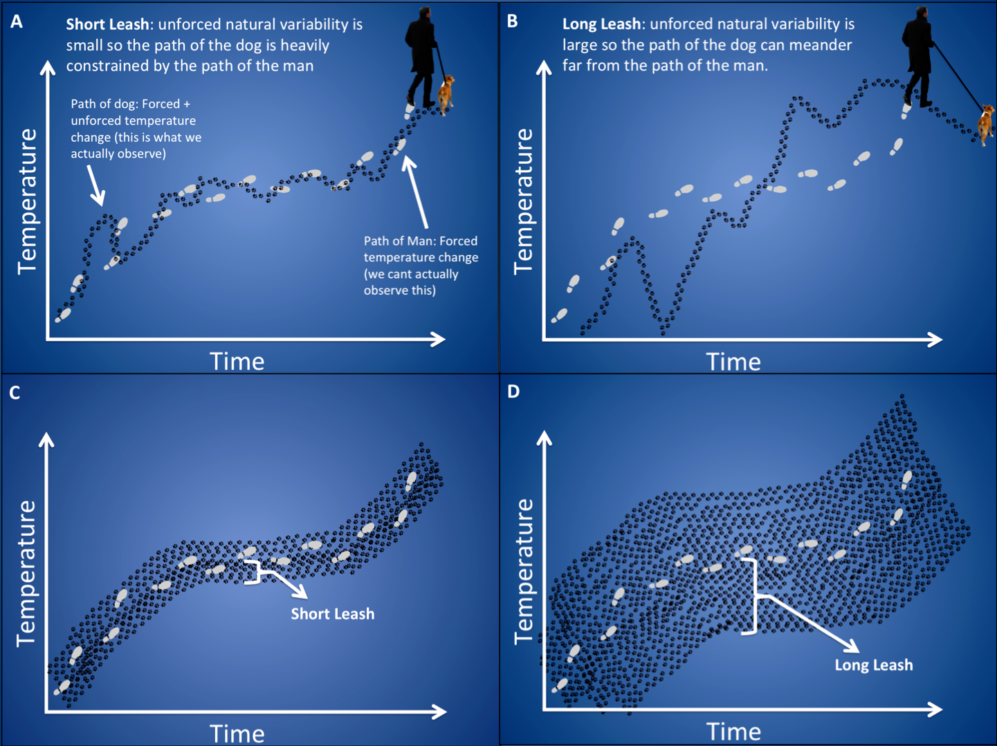
Figure 1: Man walking dog analogy for global average surface air temperature variability.
The path of the man represents forced temperature change. The path of the dog, relative to the man, represents natural unforced temperature variability. A longer leash represents the potential for larger unforced temperature variability. The path of the dog represents the actual observed temperature change, a combination of the forced (movement of man) and the unforced (movement of dog) influences on temperature change.
Determining the magnitude of unforced variability will also help us predict how global temperature might change in the future. As humans put more greenhouse gasses into the atmosphere every year, the forced temperature change will continue on his upward trajectory. If the magnitude of unforced variability is small then we should expect to see global temperatures follow this upward progression closely. However, if the magnitude of unforced variability is large, then the global temperature might deviate from the steady upward progression for decades at a time.
The most commonly used tool for determining the size of unforced natural variability is the “global climate model”. Global climate models are computer programs that use our knowledge of physics and geography to simulate the Earth’s oceanic and atmospheric circulations. Thus, these climate models actually simulate energy imbalances in order to estimate global surface temperature changes. When a climate model is run, it simulates a single possible trajectory of the temperature progression. The size of unforced variability is inferred from a computer climate model by running it many times with the same forced temperature changes but with slightly different histories of natural unforced cycles – histories that could have happened. This is analogous to figuring out the length of the leash by observing the height of the sum of the dog’s paths (Figure 1: C and D).
Our new way to estimate the size of unforced variability
Several recent studies have suggested that global climate models might underestimate the magnitude of unforced natural temperature variability ([2]; [5]; [6]). Considering this, it is valuable to estimate the size of unforced variability from an independent source. In our study, we estimated the size of unforced variability by examining the historical record of temperature change in two types of datasets. We used the “instrumental record” from the year 1880 to 2013, which represents the temperature record measured directly with thermometers. This record is relatively short, so we also used “proxy reconstructions” of temperatures from the year 1000 to 1850. Proxy reconstructions represent estimates of historical temperature that come from “natural thermometers” present in the environment. Some examples of natural thermometers include tree rings, corals, pollen, ice layers, stalactites, and lake sediments.
We used a statistical method called “Multiple Linear Regression” in order to separate forced from unforced temperature variability in these records. Our Multiple Linear Regression technique noted how much of the temperature variability in the past was correlated with changes in forcings. Any temperature variability that was correlated with changes in forcings was not counted as part of our estimate of unforced variability. We then used this estimate of unforced temperature variability to create our own simulations of unforced variability over the 20th and 21st centuries. We did this with a statistical method called “noise modeling”. Our noise modeling technique used a computer’s random number generator to create thousands of hypothetical temperature trajectories over the 20th and 21st centuries with the same amount of unforced variability as what we found in our historical datasets (Figure 2). These trajectories represented alternative histories – again the range of temperatures that could have occurred with the same forced temperature change. They were also used to represent the range of possible outcomes that we might expect to observe under future increases in greenhouse gasses. We used this new data to address two main questions:
- Is unforced natural variability large enough to account for the decade-to-decade variability in the rate of global warming over the 20th century?
- Does the reduced rate of global warming over the beginning of the 21st century indicate that forced temperature changes slowed drastically, or is unforced variability large enough to make global warming hiatus periods inevitable in the long run?
Implications of our new estimate of the size of unforced variability
We found that unforced variability is large enough to have accounted for decade-to-decade changes in the rate of global warming over the 20th century (Figure 2: B). This means that unforced variability is a little bit larger than most global climate models have traditionally indicated. However, our results made it clear that unforced temperature variability is not large enough to account for the total global warming that has been observed since 1900. Therefore, our study confirms that forced temperature changes, such as those from human-caused increases in greenhouse gasses, were necessary for the Earth to have warmed as much as it did over the past century [7].
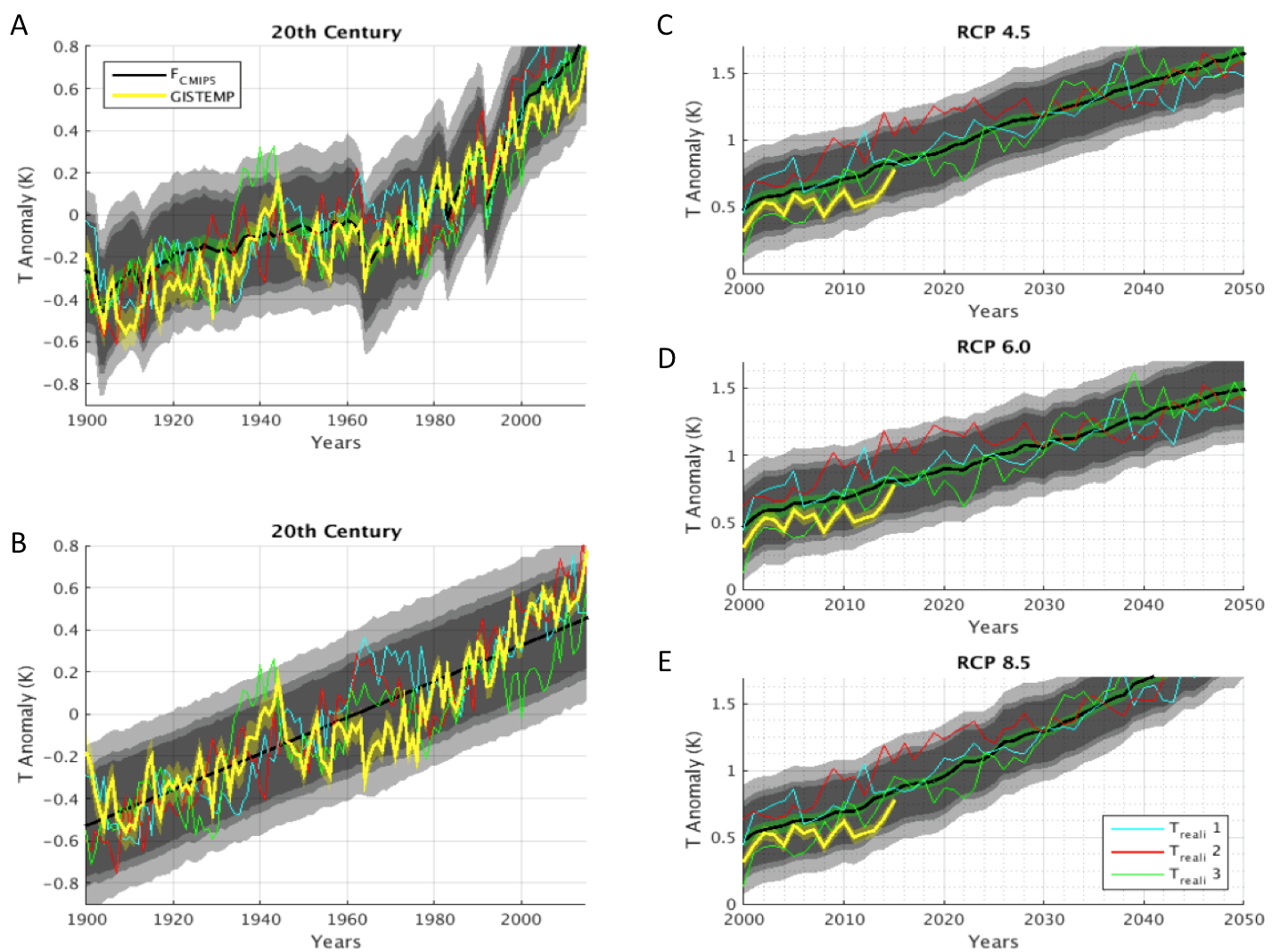
Figure 2: Estimates of forced variability and the range of unforced variability for global average temperature.
The black line represents forced variability (analogous to the path of the man in Figure 1) while the gray shading represents the range of unforced variability that we found in our study (analogous to the length of the leash in Figure 1). The yellow line is the observed temperature progression while the green, blue, and red lines represent alternative temperature progressions that could have occurred with the same forced variability but different unforced variability. Panels A and B show two different possibilities for forced variability from 1900 to 2015 while panels C, D and E show three different possibilities for forced variability over next several decades. Figure reproduced from [3].
Our findings also have implications for the first decade of the 21st century. We know that well-mixed greenhouse gasses, which cause forced temperature change, increased substantially since the turn of the century. However, global temperatures rose very little between 2002 and 2013. If unforced variability was found to be very small, the above two observations might imply that greenhouse gasses don’t cause as much warming as previously thought. However, since we found that unforced variability is relatively large, it suggests that the temperature we observe can meander substantially away from the underlying forced temperature changes. Therefore, we should not be surprised to see a period of a decade-or-so without global warming even as the forced temperature change continues on its upward trajectory (Figure 2: A). This is simply a situation where the man is progressing upward while the dog is walking down. The leash may be longer than previously thought but there is still a leash. As long as the man continues on his upward trajectory, the leash will eventually pull up on the dog (Figure 2: C, D and E) and the long term global warming trend will continue.
| [1] | P. T. Brown, W. Li, L. Li and Y. Ming: Top-of-Atmosphere Radiative Contribution to Unforced Decadal Global Temperature Variability in Climate Models, Geophysical Research Letters, https://doi.org/10.1002/2014GL060625, 2014. |
| [2] | P. T. Brown, W. Li and S. P. Xie: Regions of Significant Influence on Unforced Global Mean Surface Temperature Variability in Climate Models, Journal of Geophysical Research – Atmospheres, https://doi.org/10.1002/2014JD022576, 2015a. |
| [3] | P. T. Brown, W. Li, E. C. Cordero and S. A. Mauget: Comparing the model-simulated global warming signal to observations using empirical estimates of unforced noise, Sci. Rep., vol. 5, 2015b. |
| [4] | P. T. Brown, W. Li, J. H. Jiang and H. Su: Unforced surface air temperature variability and its contrasting relationship with the anomalous TOA energy flux at local and global spatial scales, Journal of Climate, 2016. |
| [5] | K. L. Swanson, G. Sugihara and A. A. Tsonis: Long-term natural variability and 20th century climate change, Proceedings of the National Academy of Sciences, vol. 106, 16120-16123, 2009. |
| [6] | M. G. Wyatt and J. Peters: A secularly varying hemispheric climate-signal propagation previously detected in instrumental and proxy data not detected in CMIP3 data base, SpringerPlus, vol. 1, 68, 2012. |
| [7] | N. L. Bindoff, P. A. Stott, K. M. AchutaRao, M.R. Allen, N. Gillett, D. Gutzler, K. Hansingo, G. Hegerl, Y. Hu and co-authors: Detection and Attribution of Climate Change: from Global to Regional., in: Climate Change 2013: The Physical Science Basis. Contribution of Working Group I to the Fifth Assessment Report of the Intergovernmental Panel on Climate Change. Cambridge University Press, 2013. |
