Sea level under climate change: Understanding the links between the past and the future
By Keven Roy, Nicole S. Khan, Timothy A. Shaw, Robert E. Kopp and Benjamin P. Horton, 14 January 2021
Research article
Rising global sea level, a consequence of climate change, results from an increase in the world ocean’s water volume and mass. Recent climate warming is responsible for producing the highest rate of global average sea-level rise of the past few millennia, and this rate will accelerate through the 21st century and beyond, exposing low-lying islands and coastal regions to significant flood risks. The flood risks can be compounded or diminished locally because changes in sea level are not uniform. In this review, we briefly discuss ice sheets as drivers of global and local sea levels, and how they could evolve under modern climate change. We underline some of the impacts of sea level change on coastal communities, and emphasize that local sea-level projections can be very different from estimates of the global average.
Introduction
The impacts of climate change are serious and far-reaching [IPCC, 2019]. One of its most serious consequences is the rise in global sea level that has accompanied the warming of the atmosphere and oceans and the subsequent melting of land ice. However, given the relatively slow pace of sea-level rise with respect to our daily lives, it may be easy to underestimate the gravity of its consequences on coastal populations, infrastructures and ecosystems. Here, we review how global sea level has changed in the past up to the present, the role played by ice sheets and glaciers in its evolution, and how this knowledge can be used to better understand its future.
Observations of past and modern sea-level change
To understand how sea level changes through time, various measurement techniques are used. Since the early 1990s, radars onboard satellites have been used to monitor changes in the surface of the oceans with millimetric precision [R.S. Nerem et al., 2010; H.B. Dieng et al., 2017; J.-F. Legeais et al., 2018]. To understand sea level variations further in the past, records from instruments that have been fixed along the coast to measure sea level and tides (called tide gauges) are used. Long-term trends in those records can provide information on global sea-level change, but recovering this signal is challenging, and careful consideration must be given to the baseline to which any change in sea level is assessed [J.A. Church and N.J. White, 2011; C.C. Hay et al., 2015; S. Dangendorf et al., 2019]. Although some records cover the whole 20th century and even before, most of the records are much shorter, suffer from gaps and are concentrated in the Northern Hemisphere. Therefore, careful statistical analyses are required to infer from them the global behaviour of sea level. Some examples of tide gauge records showing very different patterns of sea level change are shown in the top panels of figure 1.
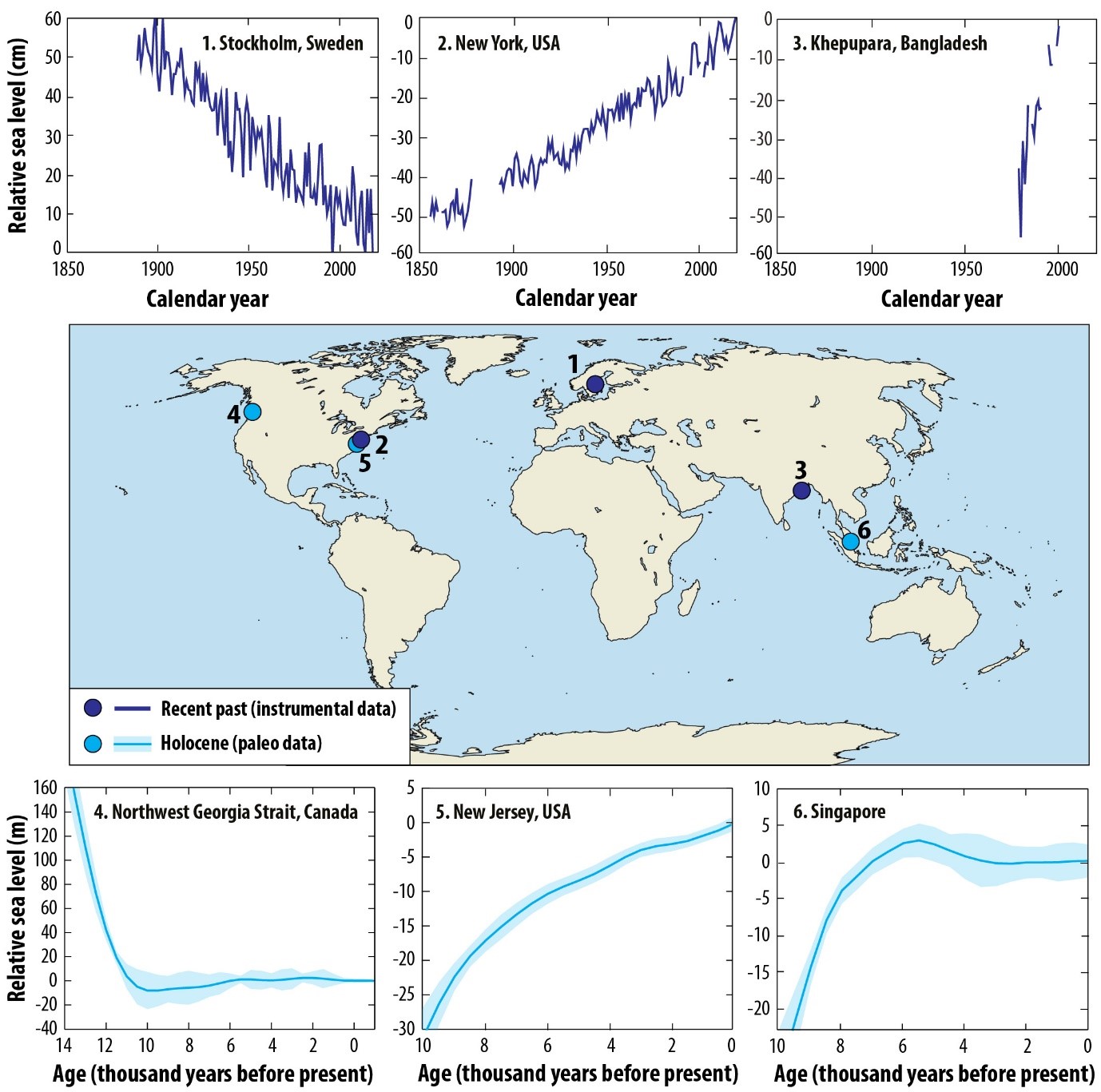
Figure 1: Examples of relative sea level change observed for the instrumental period (top panels, dark blue) and for the Holocene era (bottom panels, light blue), together with their position on a world map (middle panel). The top panels show tide gauge measurements for (1) Stockholm, Sweden (sea level fall); (2) New York, USA (sea level rise); and (3) Khepupara, Bangladesh (rapid sea level rise) [PSMSL, 2018; S.J. Holgate et al., 2013]. The bottom panels show relative sea level change in the past few thousand years using proxies, for (1) Northwest Georgia Strait, Canada [S.E. Engelhart et al., 2015]; (2) New Jersey, USA [B.P. Horton et al., 2013]; and (3) Singapore [M.I. Bird et al., 2010]. The lighter-coloured shaded area represents the uncertainty in the value of sea level (1 standard deviation). The three sites in the lower panels show the very different impact of long-term glacial isostatic adjustment between regions. Please note the different time scales (years vs. thousands of years) and amplitudes (centimetres vs. metres) used in the top and bottom panels. Modified from [N.S. Khan et al., 2015].
A clear picture has emerged from those tide gauge records. Sea levels have been increasing at an accelerating rate for most coastlines worldwide. Over the 1901-1990 period, the average increase was about 1.2 mm/year, while it rose to about 3.0 mm/year over the 1993-2010 period [C.C. Hay et al., 2015]. Estimates from satellites are consistent with tide gauge observations and indicate about 3.1 mm/year of global sea-level rise over the 1993-2018 period [WCRP, 2018]. It is estimated that the melting of mountain glaciers, of the Greenland ice sheet and of the Antarctica ice sheet have respectively contributed about 0.7, 0.5 and 0.7 mm/year to this value, while the thermal expansion of the oceans has raised global sea level by about 1.3 mm/year [WCRP, 2018]. The rest of the signal (about 0.4 mm/yr) can be linked to other changes in land water storage, such as groundwater extraction.
To understand how sea level changed before those records existed, more indirect measurement methods, called sea-level proxies, are used [B.P. Horton et al., 2018]. Such proxies have a measurable relationship to sea level, and may include wetlands flooded regularly by tides, archaeological remains of coastal structures or material deposited along former beaches [I. Shennan, 2015]. Careful measurements of the depth and age of formation of this material can be used to estimate where sea level was at a given location and time in the past. If retrieved at different ages and from different elevations, the history of local sea-level changes can be reconstructed relative to a present-day reference point (what is called relative sea level) (figure 1, bottom panels). Over many decades, a large number of records covering most coastlines have been assembled [N.S. Khan et al., 2015]. Such proxy records have reinforced the link between global climate conditions and sea level change, and demonstrate that the rate of global sea-level rise over the past century was greater than the rate during any other century over the past 3,000 years [R.E. Kopp et al., 2016; A.C. Kemp et al., 2018].
Ice sheets as drivers of sea-level change and variability
Overall, global sea-level change is driven by the mass and the volume of water contained in the oceans, but it manifests itself in an irregular manner around the world, as a range of processes overlap to create regional and local variability [R.E. Kopp et al., 2015]. At all timescales, sea level responds to tides, regional weather conditions (e.g. atmospheric pressure, evaporation/precipitation, surface winds, freshwater runoff from the land, etc.) and to any trends in wind patterns and oceanic currents, but this review focuses on the surprisingly complex contribution from ice sheet melting.
Over long timescales, a major source of sea-level variability comes from the ongoing physical response of the Earth to the last ice age. The Earth is not fully rigid, and it deforms under weights that rest on its surface. At the peak at the Last Glacial Period, more than 20,000 years ago (a period known as the Last Glacial Maximum), ice sheets covered large parts of North America and Northern Europe, in addition to the ice sheets currently covering Antarctica and Greenland [W.R. Peltier, 2004; W.R. Peltier et al., 2015; K. Roy and W.R. Peltier, 2017]. In some locations in North America, the Laurentide ice sheet reached over 4 kilometres in thickness (similar to the maximum thickness of the ice sheet currently covering Antarctica). The water locked in those ice sheets led to an average sea level that was around 120 meters lower than today. As shown the left panels of figure 2, the land located underneath the former ice sheets was pressed down under the weight of such heavy ice masses, pushing out the displaced Earth material. This uplifted the land located outside the edges of the ice sheets. When the ice started melting and returning to the oceans, the Earth’s crust began a slow return to equilibrium. This ongoing process is called glacial isostatic adjustment. As shown on the bottom left panel of figure 2, it creates distinct patterns of sea-level change that depend on where a place is located with respect to the former ice sheets, and will also be impacted by the increased weight of water contained in the oceans [N.S. Khan et al., 2015]. In regions that were covered by land ice, like northern Canada, the crust has been moving upwards leading, in some instances, to a sea level fall that is still ongoing. Conversely, the land is subsiding in regions that were located just outside the former ice sheets, such as the East Coast of the United States, leading to a faster-than-average sea level rise. In some areas, this impact can be exacerbated or dominated by tectonics and other sources of local subsidence, such as groundwater or oil/gas extraction.
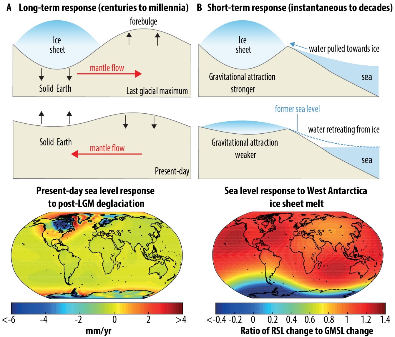
Figure 2: Schematic of two ice sheet-related drivers of sea level change over longer (left) and shorter (right) timescales, as discussed in the text. The upper left panels show a cartoon of glacial isostatic adjustment, with the vertical arrows representing land motion and the red arrows the movement of the material inside the Earth, while the bottom left panel shows a map of the vertical motion of the Earth at present in response to the deglaciation that occurred after the Last Glacial Maximum (LGM) (millimetres per year). The melting of an ice sheet impacts sea level on shorter timescales due to the increase in mass of the ocean and because of gravitational, rotational and elastic deformation effects. The upper right panel focuses on the gravitational and elastic deformation components of this response. As an example, the bottom right panel shows a map of how sea level changes in the short term from melting in West Antarctica, as a fraction of the global mean sea level (GMSL) change. Regions in blue show a fall in sea level or a much lower relative sea level rise than the global mean, while regions in red show a relative sea level rise greater than the global mean. Maps modified from [R.E. Kopp et al., 2015].
Sea-level variability is also driven by ice sheets on shorter timescales. For instance, present-day climate change has a strong impact on sea level worldwide. Satellite-based measurements of the mass balance of the Greenland and Antarctic ice sheets indicate they have respectively lost on average about 280 and 160 billion tons of ice each year over the 2006-2015 period [A. Shepherd et al., 2018; IPCC, 2019; A. Shepherd et al., 2020]. Mountain glaciers, although far less massive in total than the ice sheets, are comparatively more vulnerable to changes in temperature due to their smaller size. Measurements of their year-to-year changes are challenging, but current estimates indicate they have lost on average 220 billion tons of ice per year over 2006-2015 [IPCC, 2019]. This influx of water in the oceans leads to an increase in average sea level, but it is not uniform, as the surface of the oceans responds to changes in the planet’s gravity. As shown in the right panels of figure 2, ice sheets gravitationally attract ocean waters due to their large mass, raising sea level around them. If an ice sheet melts, its gravitational attraction decreases and, thus, sea level around it can counter-intuitively go down. Conversely, regions far from a melting ice sheet will see an increase in sea level greater than the global average. Each melting ice sheet will thus create a specific global pattern of sea-level change(1). The bottom right panel of figure 2 shows the pattern produced by a melting of Western Antarctica, which would increase sea level rise in North America by a value that is about 30% higher than the global average.
Future estimates of sea-level change
This understanding of sea-level change drivers can be combined with estimates of future greenhouse gas emissions to create models of sea-level change throughout the 21st century and beyond [B.P. Horton et al., 2018; IPCC, 2019]. Those models provide global and regional estimates of variability.
However, current projections of sea-level rise over the 21st century exhibit sizeable uncertainties. Those are mainly related to the unknown path that greenhouse gas emissions will follow and to uncertainties in the response of the ice sheets to climate change [J.L. Bamber et al., 2019]. An example of such recent projections of average sea-level rise over the 21st century and beyond is presented in figure 3. The projections to 2100 have a likely range(2) of 0.5 to 1 m under a low-emission scenario, and of between 0.8 and 1.8 m for a high-emission scenario with an unstable Antarctic ice sheet(3) [J.L. Bamber et al., 2019]. Extending those projections further into the future reveals even larger differences between the scenarios. In fact, if looking at changes until 2300, the likely range for a low-emission scenario is between 1.2 and 3.6 m but reaches between 2.7 and 6.5 m for high-emission cases [J.L. Bamber et al., 2019]. However, those values are global averages and local projections are strongly impacted by spatial variability.
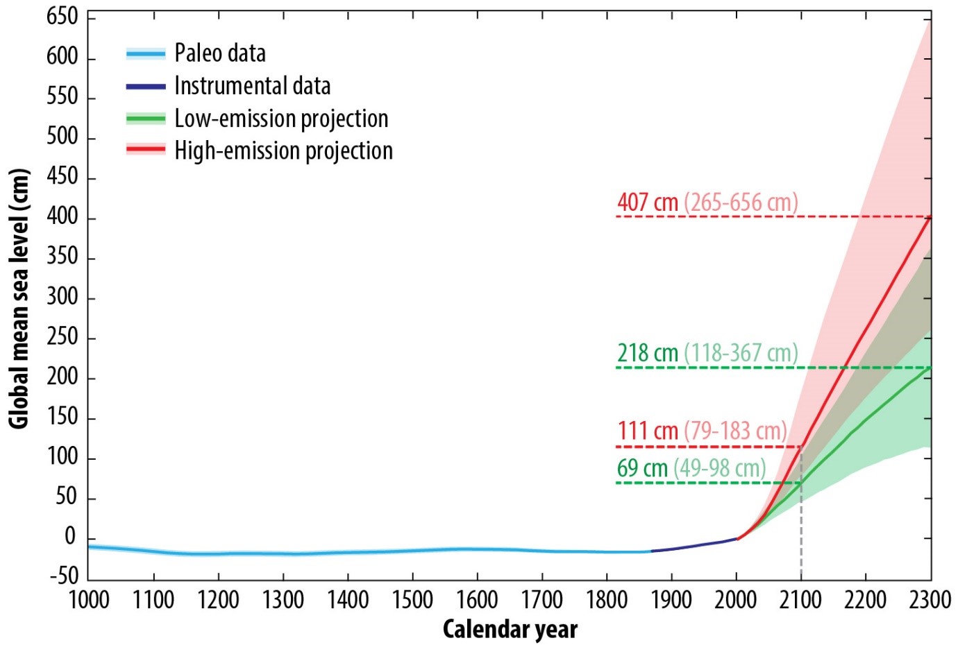
Figure 3: Change in global mean sea level measured since 1000AD using sea level proxies (blue), as well as tide gauges and satellite measurements (purple) [A.C. Kemp et al., 2018]. Projections until 2300 are shown for low (green) and high (red) carbon emission scenarios [J.L. Bamber et al., 2019]. Shaded areas show the error range corresponding to one standard deviation. All values are with respect to the mean sea level in 2000 CE. Coloured numerical values indicate the median value of mean sea level rise for each scenario (with the one standard deviation error range in parentheses).
Why does it matter?
250 million people currently live below annual flood levels, 220 million of which are found in Asia (see table 1). Low-lying islands and coastal regions with high population densities, mainly concentrated in Asia and Oceania, are extremely vulnerable to sea-level rise. For instance, the average elevation of the Maldives is below 1.5 m above mean sea level [MEE, 2017], while other island countries, such as Kiribati, Tuvalu and the Marshall Islands, lie within 2 m of mean sea level [CIA, 2018]. Other countries have a very large fraction of their population living in low-lying deltas and floodplains, particularly in Asia. For instance, 27% of Bangladesh’s population lives within 2 m of the average height of the highest local daily tide(4) [S.A. Kulp and B.H. Strauss, 2019]. This makes Asia particularly vulnerable to a rise in sea level. In fact, the 8 countries with the most population living in potentially vulnerable areas are found in Asia (5 of which in Southeast Asia)(5). The population migrations resulting from sea level rise could potentially have geopolitical repercussions and are seen by various military organizations as a risk for global security in the 21st century [House Armed Services Committee, 2014; HM Government, 2015].
| Region | Year 2000 | Year 2100 | ||
|---|---|---|---|---|
| Low emissions | High emissions | High emissions + Antarctica instability |
||
| Asia | 220 | 322 | 347 | 421 |
| Eastern Asia | 89.6 | 123 | 136 | 165 |
| Southeast Asia | 66.5 | 94 | 100 | 124 |
| Southern Asia | 59.9 | 101 | 106 | 125 |
| Western Asia | 3.52 | 4.81 | 5.17 | 7.63 |
| Europe | 12.2 | 15.4 | 16.6 | 21.7 |
| Africa | 10.5 | 11.7 | 14.4 | 19.3 |
| South America | 2.71 | 4.12 | 4.75 | 8.36 |
| North America | 1.87 | 3.42 | 3.94 | 6.96 |
| Oceania | 0.45 | 0.81 | 0.97 | 1.82 |
| Central America | 0.35 | 0.55 | 1.09 | 2.48 |
| World (total) | 251 | 362 | 392 | 484 |
Table 1: Estimated population (in millions) exposed to local 1-year coastal flood return level in 2000 and in 2100 for various projections(6).
Beyond the permanent flooding of low-lying coastal regions, sea-level rise will also expose new areas to recurrent tidal flooding or potential storm surges [IPCC, 2019]. The height of flooding attained during a storm is the product of the storm-surge height, the timing in the astronomical tidal cycle and the local wave and surface conditions, all superimposed on the local background sea level. A change in background sea level will shift the distribution of potential extreme events, with a disproportionate impact on the return period of unlikely tail events. As coastal engineers should consider the worst-case flood scenarios that could impact coastal infrastructures during their lifetime, any change in the frequency of extreme events can overwhelm existing sea wall barriers meant to protect coastal communities, even if they remain above mean sea level.
Large fractions of the United States coastline have been found to be very susceptible to worsening flood risk. A recent study determined that local flood heights corresponding to ‘100-year events’ (flood levels that have a 1% change of being reached or exceeded in any given year) would be matched or surpassed more frequently by 2050 (median 40-fold increase in frequency), with significant differences between regions because of spatial variability in sea level rise [M.K. Buchanan et al., 2017]. Another specific example comes from Hurricane Sandy, which hit the East coast of the United States with force in 2012 (in particular New York City and New Jersey). The large storm surge that hit the region (3.5 m above mean tidal level(7)) was responsible for a large fraction of the estimated 68 billion US dollars in total economic loss [Impact Forecasting, 2013]. In New York City, where sea level has risen by around 46 cm since 1856, the return period of the pre-industrial 500-year return period storm surge (2.25 m above mean tidal level [A.J. Reed et al., 2015]) has been reduced to 25 years for the 1970-2005 period. Current projections of sea-level rise indicate that this return period could go down to 5 years by 2030-2045. In consequence, while a 2.25 m surge height had a yearly probability of occurrence of 0.2% in the pre-industrial era, this probability could go up to 20% by 2030-2045 [A.J. Garner et al., 2017].
Sea level change has an important impact on coastal ecosystems and the natural services they provide. Marsh and mangrove ecosystems provide protection against coastal erosion, as they trap sediments, attenuate waves and stabilise shorelines. Tidal wetlands can keep up vertically with sea level rise if the rate of change is within the range of sediment build-up that can sustain the ecosystem. For mangroves, recent analyses suggest that this threshold is about 7 millimetres per year, a rate which could be reached within 30 years for many tropical coastlines [N. Saintilan et al., 2020]. Sea-level rise will also impact water and food security, due to saltwater intrusions in low-lying water tables and in agriculture-intensive flood plains [S. Adams et al., 2013]. Low-lying deltas are particularly vulnerable: for the Mekong delta, which generates 20% of the global rice trade, some studies estimate that the combined impacts of soil elevation and salinity changes could lead to a 50% decrease in rice field productivity by 2100 under high-emission scenarios [A. Smajgl et al., 2015]. Early indications of increased salinity levels due to sea level rise have already been documented in some estuaries, such as Chesapeake Bay in Delaware, USA [A.C. Ross et al., 2015].
Conclusion
The rise in global sea level brought by climate change is a serious societal concern, due to the hazard it poses to coastal populations, infrastructures and ecosystems. Multiple factors influence how sea level rise manifests itself locally and many areas will suffer from disproportionate impacts. The relatively slow response of ice sheets to elevated levels of greenhouse gases, as well as the fact that a small change in mean sea level can still have a significant impact on the local frequency of extreme water levels, are important features of a changing climate. Understanding them is essential in designing appropriate adaptation measures for coastal communities.
| (1) | This pattern is referred to as a ‘sea-level fingerprint’ or ‘Barystatic-GRD fingerprint’, arising from the increase in mass of the ocean (barystatic) and gravitational, rotational and elastic deformation impacts (GRD) [J.M. Gregory et al., 2019]. |
| (2) | Defined as the range between the 17th and 83rd percentiles. |
| (3) | The emission scenarios discussed here are from [J.L. Bamber et al., 2019]. The ‘low-emission’ and ‘high-emission’ scenarios refer to a global mean warming in 2081-2100 of +1.9°C and +4.5°C above pre-industrial levels, respectively. |
| (4) | Also referred to as ‘Mean Higher High Water’ (MHHW). |
| (5) | The top 10 is formed of China (110), Bangladesh (43), India (42), Vietnam (39), Indonesia (33), Japan (16), Thailand (14), the Philippines (12), the Netherlands (7) and Egypt (5.8). Based on the data from [S.A. Kulp and B.H. Strauss, 2019] for the population living below 2 m above MHHW (shown in parentheses, in millions). |
| (6) | Based on [S.A. Kulp and B.H. Strauss, 2019], and using geographical region definitions from the World Bank. The numbers for 2100 are based, for the ‘Low emissions’ and ‘High emissions’ cases, on the median of the probability distribution of future sea level rise from [R.E. Kopp et al., 2014], while the ‘High emissions + Antarctica instability’ case is based on the median frequency distribution from [R.E. Kopp et al., 2017]. |
| (7) | Mean tidal level is the difference between the mean high water and mean low water, measured here at the Battery tide gauge in New York City. |
| [1] | S. Adams, F. Baarsch, A. Bondeau, D. Coumou, R. Donner, K. Frieler, B. Hare, A. Menon, M. Perette and co-authors: Turn down the heat : climate extremes, regional impacts, and the case for resilience – full report (English), World Bank, 254 pp., 2013. |
| [2] | J.L. Bamber, M. Oppenheimer, R.E. Kopp, W.P. Aspinall and R.M. Cooke: Ice sheet contributions to future sea-level rise from structured expert judgment, in: Proceedings of the National Academy of Sciences of the United States of America, 11195-11200, https://doi.org/10.1073/pnas.1817205116, 2019. |
| [3] | M.I. Bird, W.E.N. Austin, C.M. Wurster, L.K. Fifield, M. Mojtahid and C. Sargeant: Punctuated eustatic sea-level rise in the early mid-Holocene, Geology, vol. 38(9), 803-806, https://doi.org/10.1130/G31066.1, 2010. |
| [4] | M.K. Buchanan, M. Oppenheimer and R.E. Kopp: Amplification of flood frequencies with local sea level rise and emerging flood regimes, Environmental Research Letters, vol. 12(6), 064009, https://doi.org/10.1088/1748-9326/aa6cb3, 2017. |
| [5] | J.A. Church and N.J. White: Sea-Level Rise from the Late 19th to the Early 21st Century, Surveys in Geophysics, vol. 32(4-5), 585-602, https://doi.org/10.1007/s10712-011-9119-1, 2011. |
| [6] | CIA: The World Factbook . Central Intelligence Agency. Retrieved (2018) from https://www.cia.gov/library/publications/the-world-factbook/index.html. |
| [7] | House Armed Services Committee: The 2014 Quadrennial Defense Review: Committee on Armed Services, House of Representatives, One Hundred Thirteenth Congress, Second Session, 88 pp., 2014. |
| [8] | S. Dangendorf, C. Hay, F.M. Calafat, M. Marcos, C.G. Piecuch, K. Berk and J. Jensen: Persistent acceleration in global sea-level rise since the 1960s, Nature Climate Change, vol. 9, 705-710, https://doi.org/10.1038/s41558-019-0531-8, 2019. |
| [9] | H.B. Dieng, A. Cazenave, B. Meyssignac and M. Ablain: New estimate of the current rate of sea level rise from a sea level budget approach, Geophysical Research Letters, vol. 44, 3744-3751, https://doi.org/10.1002/2017GL073308, 2017. |
| [10] | S.E. Engelhart, M. Vacchi, B.P. Horton, A.R. Nelson and R.E. Kopp: A sea-level database for the Pacific coast of central North America, Quaternary Science Reviews, vol. 113(1), 78-92, https://doi.org/10.1016/j.quascirev.2014.12.001, 2015. |
| [11] | Impact Forecasting: Hurricane Sandy Event Recap Report, Aon Benfield, 50pp pp., 2013. Retrieved from http://thoughtleadership.aonbenfield.com/Documents/20130514_if_hurricane_sandy_event_recap.pdf. |
| [12] | A.J. Garner, M.E. Mann, K.A. Emanuel, R.E. Kopp, N. Lin, R.B. Alley, B.P. Horton, R.M. DeConto, J.P. Donnelly and co-authors: Impact of climate change on New York City’s coastal flood hazard: Increasing flood heights from the preindustrial to 2300 CE, Proceedings of the National Academy of Sciences of the United States of America, vol. 114(45), 11861-11866, https://doi.org/10.1073/pnas.1703568114, 2017. |
| [13] | HM Government: National Security Strategy and Strategic Defence and Security Review 2015: A Secure and Prosperous United Kingdom, HM Government, 98 pp., 2015. |
| [14] | J.M. Gregory, S.M. Griffies, C.W. Hughes, J.A. Lowe, J.A. Church, I. Fukimori, N. Gomez, R.E. Kopp, F. Landerer and co-authors: Concepts and terminology for sea level: Mean, variability and change, both local and global, Surveys in Geophysics, vol. 40, 1251-1289, https://doi.org/10.1007/s10712-019-09525-z, 2019. |
| [15] | C.C. Hay, E. Morrow, R.E. Kopp and J.X. Mitrovica: Probabilistic reanalysis of twentieth-century sea-level rise, Nature, vol. 517(7535), 481-484, https://doi.org/10.1038/nature14093, 2015. |
| [16] | S.J. Holgate, A. Matthews, P.L. Woodworth, L.J. Rickards, M.E. Tamisiea, E. Bradshaw, P.R. Foden, K.M. Gordon, S. Jevrejeva and co-authors: New Data Systems and Products at the Permanent Service for Mean Sea Level, Journal of Coastal Research, vol. 29(3), 493-504, https://doi.org/10.2112/JCOASTRES-D-12-00175.1, 2013. |
| [17] | B.P. Horton, S.E. Engelhart, D.F. Hill, A.C. Kemp, D. Nikitina, K.G. Miller and W.R. Peltier: Influence of tidal-range change and sediment compaction on Holocene relative sea-level change in New Jersey, USA, Journal of Quaternary Science, vol. 28(4), 403-411, https://doi.org/10.1002/jqs.2634, 2013. |
| [18] | B.P. Horton, R.E. Kopp, A.J. Garner, C.C. Hay, N.S. Khan, K. Roy and T.A. Shaw: Mapping sea-level change in time, space, and probability, Annual Review of Environment and Resources, vol. 43, 481-521, https://doi.org/10.1146/annurev-environ-102017-025826, 2018. |
| [19] | B.P. Horton, I. Shennan, S.L. Bradley, N. Cahill, M. Kirwan, R.E. Kopp and T.A. Shaw: Predicting marsh vulnerability to sea-level rise using Holocene relative sea-level data, Nature Communications, vol. 9, 2687, https://doi.org/10.1038/s41467-018-05080-0, 2018. |
| [20] | IPCC: IPCC Special Report on the Ocean and Cryosphere in a Changing Climate, H.-O. Pörtner, D.C. Roberts, V. Masson-Delmotte, P. Zhai, M. Tignor, E. Poloczanska, K. Mintenbeck, A. Alegría, M. Nicolai and co-editors (Eds.). Cambridge University Press, In press pp., 2019. |
| [21] | A.C. Kemp, A.J. Wright, R.J. Edwards, R.L. Barnett, M.J. Brain, R.E. Kopp, N. Cahill, B.P. Horton, D.J. Charman and co-authors: Relative sea-level change in Newfoundland, Canada during the past ∼3000 years, Quaternary Science Reviews, vol. 201, 89-110, https://doi.org/10.1016/j.quascirev.2018.10.012, 2018. |
| [22] | N.S. Khan, E. Ashe, T.A. Shaw, M. Vacchi and J. Walker: Holocene relative sea-level changes from near-, intermediate- and far-field locations, Current Climate Change Reports, vol. 1, 247-262, https://doi.org/10.1007/s40641-015-0029-z, 2015. |
| [23] | R.E. Kopp, R.M. DeConto, D.A. Bader, Hay, C.C., R.M. Horton, S. Kulp, M. Oppenheimer, D. Pollard and co-authors: Evolving Understanding of Antarctic Ice-Sheet Physics and Ambiguity in Probabilistic Sea-Level Projections, Earth’s Future, vol. 5(12), 1217-1233, https://doi.org/10.1002/2017EF000663, 2017. |
| [24] | R.E. Kopp, C.C. Hay, C.M. Little and J.X. Mitrovica: Geographic Variability of Sea-Level Change, Current Climate Change Reports, vol. 1(3), 192-204, https://doi.org/10.1007/s40641-015-0015-5, 2015. |
| [25] | R.E. Kopp, R.M. Horton, C.M. Little, J.X. Mitrovica, M. Oppenheimer, D.J. Rasmussen, B.H. Strauss and C. Tebaldi: Probabilistic 21st and 22nd century sea-level projections at a global network of tide-gauge sites, Earth’s Future, vol. 2(8), 383-406, https://doi.org/10.1002/2014EF000239, 2014. |
| [26] | R.E. Kopp, A.C. Kemp, K. Bittermann, B.P. Horton, J.P. Donnelly, W.R. Gehrels, C.C. Hay, J.X. Mitrovica, E.D. Morrow and co-authors: Temperature-driven global sea-level variability in the Common Era, in: Proceedings of the National Academy of Sciences of the United States of America, E1434-E1441, https://doi.org/10.1073/pnas.1517056113, 2016. |
| [27] | S.A. Kulp and B.H. Strauss: New elevation data triple estimates of global vulnerability to sea-level rise and coastal flooding, Nature Communications, vol. 10, 4844, https://doi.org/10.1038/s41467-019-12808-z, 2019. |
| [28] | J.-F. Legeais, M. Ablain, L. Zawadzki, H. Zuo, J.A. Johannessen, M.G. Scharffenberg, L. Fenoglio-Marc, M.J. Fernandes, O.B. Anderson and co-authors: An improved and homogeneous altimeter sea level record from the ESA Climate Change Initiative, Earth System Science Data Discussions, vol. 10, 281-301, https://doi.org/10.5194/essd-10-281-2018, 2018. |
| [29] | MEE: State of the Environment 2016, Ministry of Environment and Energy of the Republic of the Maldives, 216 pp., 2017. |
| [30] | R.S. Nerem, D.P. Chambers, C. Choe and G.T. Mitchum: Estimating Mean Sea Level Change from the TOPEX and Jason Altimeter Missions, Marine Geodesy, vol. 33(1), 435-446, https://doi.org/10.1080/01490419.2010.491031, 2010. |
| [31] | W.R. Peltier: Global Glacial Isostasy and the Surface of the Ice-Age Earth: The ICE-5G (VM2) Model and GRACE, Annual Review of Earth and Planetary Sciences, vol. 32, 111-149, https://doi.org/10.1146/annurev.earth.32.082503.144359, 2004. |
| [32] | W.R. Peltier, D.F. Argus and R. Drummond: Space geodesy constrains ice age terminal deglaciation: The global ICE-6G_C (VM5a) model, Journal of Geophysical Research – Solid Earth, vol. 120(1), 450-487, https://doi.org/10.1002/2014JB011176, 2015. |
| [33] | PSMSL: Permanent Service for Mean Sea Level: Tide Gauge Data. Retrieved (2018) from http://www.psmsl.org/data/obtaining. |
| [34] | A.J. Reed, M.E. Mann, K.A. Emanuel, N. Lin, B.P. Horton, A.C. Kemp and J.P. Donnelly: Increased threat of tropical cyclones and coastal flooding to New York City during the anthropogenic era, in: Proceedings of the National Academy of Sciences of the United States of America, 12610-12615, https://doi.org/10.1073/pnas.1513127112, 2015. |
| [35] | A.C. Ross, R.G. Najjar, M. Li, M.E. Mann, S.E. Ford and B. Katz: Sea-level rise and other influences on decadal-scale salinity variability in a coastal plain estuary, Estuarine, Coastal and Shelf Science, vol. 157, 79-92, https://doi.org/10.1016/j.ecss.2015.01.022, 2015. |
| [36] | K. Roy and W.R. Peltier: Space-geodetic and water level gauge constraints on continental uplift and tilting over North America: regional convergence of the ICE-6G_C (VM5a/VM6) models, Geophysical Journal International, vol. 210(2), 1115-1142, https://doi.org/10.1093/gji/ggx156, 2017. |
| [37] | N. Saintilan, N.S. Khan, E. Ashe, J.J. Kelleway, K. Rogers, C.D. Woodroffe and B.P. Horton: Thresholds of mangrove survival under rapid sea level rise, Science, vol. 368(6495), 1118-1121, https://doi.org/10.1126/science.aba2656, 2020. |
| [38] | I. Shennan: Handbook of sea-level research, in: Handbook of Sea-Level Research (ed. 1st), I. Shennan, A.J. Long and B.P. Horton (Eds.). John Wiley & Sons, 3-25, 2015. |
| [39] | A. Shepherd, E. Ivins, E. Rignot, B. Smith, den Broeke M. van, I. Velicogna, P. Whitehouse, K. Briggs, I. Joughin and co-authors: Mass balance of the Antarctic Ice Sheet from 1992 to 2017, Nature, vol. 558, 219-222, https://doi.org/10.1038/s41586-018-0179-y, 2018. |
| [40] | A. Shepherd, E. Ivins, E. Rignot, B. Smith, den Broeke M. van, I. Velicogna, P. Whitehouse, K. Briggs, I. Joughin and co-authors: Mass balance of the Greenland Ice Sheet from 1992 to 2018, Nature, vol. 579, 233-239, https://doi.org/10.1038/s41586-019-1855-2, 2020. |
| [41] | A. Smajgl, T.Q. Toan, D.K. Nhan, J. Ward, N.H. Trung, L.Q. Tri, V.P.D. Tri and P.T. Vu: Responding to rising sea levels in the Mekong Delta, Nature Climate Change, vol. 5, 167-174, https://doi.org/10.1038/nclimate2469, 2015. |
| [42] | WCRP: Global Sea Level Budget Group: Global sea-level budget 1993–present, Earth Syst. Sci. Data, vol. 10, 1551–1590, https://doi.org/10.5194/essd-10-1551-2018, 2018. |
